Dataset
To illustrate the Coralysis reference-mapping method, we
will use in this vignette two 10X PBMCs (Peripheral Blood Mononuclear
Cells) 3’ assays: V1 and V2. The assay
V2 will be the reference and
V1 the query, i.e., the dataset that will be
mapped against the reference. The datasets have been downloaded from 10X
website. The PBMC dataset V1 corresponds to sample
pbmc6k and V2 to pbmc8k:
Cells were annotated using the annotations provided by Korsunsky et
al., 2019 (Source Data Figure 4 file). The overall data was
downsampled to 2K cells (1K per assay) and 2K highly variable genes
selected with scran R package. To facilitate the
reproduction of this vignette, the data is distributed through
Zenodo as a SingleCellExperiment object, the
object (class) required by most functions in Coralysis (see
Chapter
4 The SingleCellExperiment class - OSCA manual). The
SCE object provided comprises counts (raw
count data), logcounts (log-normalized data) and cell
colData (which includes batch and cell labels, designated
as batch and cell_type, respectively).
Run the code below to import the R packages and data
required to reproduce this vignette.
# Packages
library("ggplot2")
library("Coralysis")
library("SingleCellExperiment")
# Import data from Zenodo
data.url <- "https://zenodo.org/records/14845751/files/pbmc_10Xassays.rds?download=1"
pbmc_10Xassays <- readRDS(file = url(data.url))

# Split the SCE object by assay
ref <- pbmc_10Xassays[,pbmc_10Xassays$batch=="V2"] # let V2 assay batch be the reference data set
query <- pbmc_10Xassays[,pbmc_10Xassays$batch=="V1"] # let V1 be the query (unknown annotations)
Train reference
The first step in performing reference mapping with
Coralysis is training a dataset that is representative of
the biological system under study. In this example, ref and
query correspond to the SingleCellExperiment
objects of the reference and query PBMC samples, V2 and
V1 3’ assays, respectively. The reference ref is
trained through RunParallelDivisiveICP function without
providing a batch.label. In case the reference requires
integration, a batch.label should be provided. An higher
number of threads can be provided to speed up computing
time depending on the number of cores available. For this example, the
algorithm was run 10 times (L = 10), but generally, this
number should be higher (with the default being L = 50).
Next, run the function RunPCA to obtain the main result
required for cell type prediction later on. In addition to cell type
prediction, the query dataset(s) can be projected onto UMAP. To allow
this, the argument return.model should be set to
TRUE in both functions RunPCA and
RunUMAP.
# Train the reference
set.seed(123)
ref <- RunParallelDivisiveICP(object = ref, L = 10, threads = 2) # runs without 'batch.label'
## WARNING: Setting 'divisive.method' to 'cluster' as 'batch.label=NULL'.
## If 'batch.label=NULL', 'divisive.method' can be one of: 'cluster', 'random'.##
## Building training set...## Training set successfully built.##
## Computing cluster seed.##
## Initializing divisive ICP clustering...## | | | 0% | |======== | 11% | |================ | 22% | |======================= | 33% | |=============================== | 44% | |======================================= | 56% | |=============================================== | 67% | |====================================================== | 78% | |============================================================== | 89% | |======================================================================| 100%##
## Divisive ICP clustering completed successfully.##
## Predicting cell cluster probabilities using ICP models...## Prediction of cell cluster probabilities completed successfully.##
## Multi-level integration completed successfully.
# Compute reference PCA
ref <- RunPCA(ref, return.model = TRUE, pca.method = "stats")
## Divisive ICP: selecting ICP tables multiple of 4Below is the UMAP plot for the reference sample with cell type annotations. In this example, we are using the annotations provided in the object. Ideally, the sample should be annotated after training by performing clustering and manual cluster annotation. Only the resulting manual cell type annotations should be used for prediction. For simplicity, we will use the annotations provided in the object.
# Vizualize reference
ref.celltype.plot <- PlotDimRed(object = ref,
                                color.by = "cell_type",
                                dimred = "UMAP",
                                point.size = 0.01,
                                legend.nrow = 6,
                                seed.color = 7) +
    ggtitle("reference (ground-truth)")
ref.celltype.plot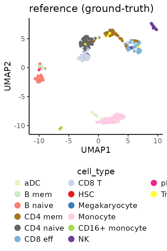
Map query
Perform reference-mapping with Coralysis by running the
function ReferenceMapping. This requires to provide the
trained reference (ref) with cell type annotations intended
for the prediction (ref.label = "cell_type") and the query
dataset (query). The label in the reference aimed to be
used for prediction needs to be available on colData(ref).
In this case, we are providing the cell type labels from the column
cell_type available in the reference ref.
Since we want to project the query onto the reference UMAP, set
project.umap as TRUE. The argument
dimred.name.prefix just sets the name given as prefix of
the low dimensional embeddings stored in
reducedDimNames(map). The SingleCellExperiment
object map will contain the same information as
query, with the predictions and embeddings mapped onto the
reference. The predictions consist in coral_labels and
coral_probability stored in colData(map). The
coral_labels correspond to the cell type predictions
obtained against the reference. The coral_probability
represents the proportion of K neighbors from the winning class
(k.nn equal 10 by default); the higher the value, the
better.
## Reference-mapping
set.seed(1024)
map <- ReferenceMapping(ref = ref, query = query, ref.label = "cell_type",
                        project.umap = TRUE, dimred.name.prefix = "ref")
Prediction accuracy
The accuracy of Coralysis reference-mapping method is
presented below together with a confusion matrix between the predicted
(rows) versus ground-truth cell type labels (columns).
Confusion matrix
# Confusion matrix
preds_x_truth <- table(map$coral_labels, map$cell_type)
stopifnot(all(row.names(preds_x_truth)==colnames(preds_x_truth)))

# Accuracy
acc <- sum(diag(preds_x_truth)) / sum(preds_x_truth)
#print(paste0("Prediction accuracy: ", acc*100, "%"))

# Print confusion matrix
preds_x_truth
##
## aDC B mem B naive CD4 mem CD4 naive CD8 eff CD8 T HSC
## aDC 14 0 0 0 0 0 0 0
## B mem 0 40 15 0 0 0 0 3
## B naive 0 4 69 0 0 0 0 0
## CD4 mem 0 0 0 108 39 3 6 0
## CD4 naive 0 0 0 14 153 0 12 2
## CD8 eff 0 1 0 2 0 93 2 0
## CD8 T 0 0 1 3 4 11 62 0
## HSC 0 0 0 0 0 0 0 0
## Megakaryocyte 0 0 0 0 0 0 0 0
## Monocyte 1 0 0 0 0 0 0 0
## CD16+ monocyte 0 0 0 0 0 0 0 0
## NK 0 0 0 0 0 1 0 0
## pDC 0 0 0 0 0 0 0 0
## Treg 0 0 0 1 0 0 0 0
##
## Megakaryocyte Monocyte CD16+ monocyte NK pDC Treg
## aDC 0 0 0 0 0 0
## B mem 0 0 0 0 0 0
## B naive 0 0 0 0 1 0
## CD4 mem 0 0 0 0 0 8
## CD4 naive 0 0 0 0 0 7
## CD8 eff 1 0 0 1 0 0
## CD8 T 1 0 0 0 0 0
## HSC 0 0 0 0 0 0
## Megakaryocyte 0 0 0 0 0 0
## Monocyte 3 173 4 1 0 0
## CD16+ monocyte 1 5 72 0 0 0
## NK 0 0 0 55 0 0
## pDC 0 0 0 0 3 0
## Treg 0 0 0 0 0 0The accuracy of Coralysis reference-mapping method was
84.2%.
DimRed
Visualize below the query cells projected onto reference UMAP and how
well the predictions match the query ground-truth. The
coral_probability is a prediction confidence score.
Predictions with low scores (<0.5) should be carefully inspected.
# Plot query and reference UMAP side-by-side
#with ground-truth & predicted cell labels
use.color <- c("aDC" = "#E6F5C9",
               "B mem" = "#CCEBC5",
               "B naive" = "#FB8072",
               "CD4 mem" = "#A6761D",
               "CD4 naive" = "#666666",
               "CD8 eff" = "#80B1D3",
               "CD8 T" = "#CBD5E8",
               "HSC" = "#E31A1C",
               "Megakaryocyte" = "#377EB8",
               "Monocyte" = "#FCCDE5",
               "CD16+ monocyte" = "#A6D854",
               "NK" = "#6A3D9A",
               "pDC" = "#E7298A",
               "Treg" = "#FFFF33")
query.ground_truth.plot <- PlotDimRed(object = map,
                                      color.by = "cell_type",
                                      dimred = "refUMAP",
                                      point.size = 0.01,
                                      legend.nrow = 6,
                                      seed.color = 7) +
    ggtitle("query (ground-truth)")
query.predicted.plot <-PlotDimRed(object = map,
                                  color.by = "coral_labels",
                                  dimred = "refUMAP", point.size = 0.01,
                                  legend.nrow = 6,
                                  use.color = use.color) +
    ggtitle("query (predicted)")
query.confidence.plot <- PlotExpression(object = map,
                                        color.by = "coral_probability",
                                        dimred = "refUMAP",
                                        point.size = 0.01,
                                        color.scale = "viridis") +
    ggtitle("query (confidence)")
cowplot::plot_grid(ref.celltype.plot, query.ground_truth.plot,
                   query.predicted.plot, query.confidence.plot,
                   ncol = 2, align = "vh")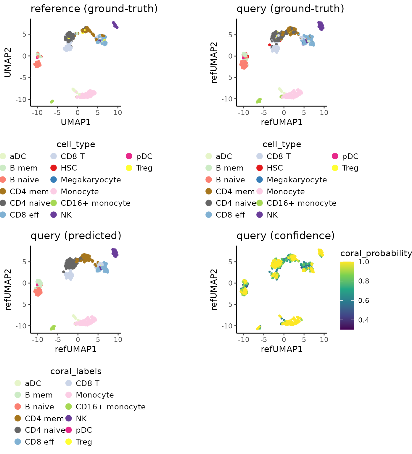
R session
# R session
sessionInfo()
## R version 4.4.2 (2024-10-31)
## Platform: x86_64-pc-linux-gnu
## Running under: Ubuntu 24.04.1 LTS
##
## Matrix products: default
## BLAS: /usr/lib/x86_64-linux-gnu/openblas-pthread/libblas.so.3
## LAPACK: /usr/lib/x86_64-linux-gnu/openblas-pthread/libopenblasp-r0.3.26.so; LAPACK version 3.12.0
##
## locale:
## [1] LC_CTYPE=C.UTF-8 LC_NUMERIC=C LC_TIME=C.UTF-8
## [4] LC_COLLATE=C.UTF-8 LC_MONETARY=C.UTF-8 LC_MESSAGES=C.UTF-8
## [7] LC_PAPER=C.UTF-8 LC_NAME=C LC_ADDRESS=C
## [10] LC_TELEPHONE=C LC_MEASUREMENT=C.UTF-8 LC_IDENTIFICATION=C
##
## time zone: UTC
## tzcode source: system (glibc)
##
## attached base packages:
## [1] stats4 stats graphics grDevices utils datasets methods
## [8] base
##
## other attached packages:
## [1] SingleCellExperiment_1.28.1 SummarizedExperiment_1.36.0
## [3] Biobase_2.66.0 GenomicRanges_1.58.0
## [5] GenomeInfoDb_1.42.3 IRanges_2.40.1
## [7] S4Vectors_0.44.0 BiocGenerics_0.52.0
## [9] MatrixGenerics_1.18.1 matrixStats_1.5.0
## [11] Coralysis_1.0.0 ggplot2_3.5.1
##
## loaded via a namespace (and not attached):
## [1] rlang_1.1.5 magrittr_2.0.3 flexclust_1.4-2
## [4] compiler_4.4.2 png_0.1-8 systemfonts_1.2.1
## [7] vctrs_0.6.5 reshape2_1.4.4 stringr_1.5.1
## [10] pkgconfig_2.0.3 crayon_1.5.3 fastmap_1.2.0
## [13] XVector_0.46.0 labeling_0.4.3 scuttle_1.16.0
## [16] rmarkdown_2.29 ggbeeswarm_0.7.2 UCSC.utils_1.2.0
## [19] ragg_1.3.3 xfun_0.50 modeltools_0.2-23
## [22] bluster_1.16.0 zlibbioc_1.52.0 cachem_1.1.0
## [25] beachmat_2.22.0 jsonlite_1.8.9 DelayedArray_0.32.0
## [28] BiocParallel_1.40.0 irlba_2.3.5.1 parallel_4.4.2
## [31] aricode_1.0.3 cluster_2.1.6 R6_2.6.0
## [34] bslib_0.9.0 stringi_1.8.4 RColorBrewer_1.1-3
## [37] reticulate_1.40.0 limma_3.62.2 jquerylib_0.1.4
## [40] Rcpp_1.0.14 iterators_1.0.14 knitr_1.49
## [43] snow_0.4-4 Matrix_1.7-1 igraph_2.1.4
## [46] tidyselect_1.2.1 abind_1.4-8 yaml_2.3.10
## [49] codetools_0.2-20 doRNG_1.8.6.1 lattice_0.22-6
## [52] tibble_3.2.1 plyr_1.8.9 withr_3.0.2
## [55] askpass_1.2.1 ggrastr_1.0.2 evaluate_1.0.3
## [58] desc_1.4.3 pillar_1.10.1 rngtools_1.5.2
## [61] foreach_1.5.2 generics_0.1.3 sparseMatrixStats_1.18.0
## [64] munsell_0.5.1 scales_1.3.0 class_7.3-22
## [67] glue_1.8.0 metapod_1.14.0 pheatmap_1.0.12
## [70] LiblineaR_2.10-24 tools_4.4.2 BiocNeighbors_2.0.1
## [73] ScaledMatrix_1.14.0 SparseM_1.84-2 RSpectra_0.16-2
## [76] locfit_1.5-9.11 RANN_2.6.2 fs_1.6.5
## [79] scran_1.34.0 Cairo_1.6-2 cowplot_1.1.3
## [82] grid_4.4.2 umap_0.2.10.0 edgeR_4.4.2
## [85] colorspace_2.1-1 GenomeInfoDbData_1.2.13 beeswarm_0.4.0
## [88] BiocSingular_1.22.0 vipor_0.4.7 cli_3.6.3
## [91] rsvd_1.0.5 textshaping_1.0.0 viridisLite_0.4.2
## [94] S4Arrays_1.6.0 dplyr_1.1.4 doSNOW_1.0.20
## [97] gtable_0.3.6 sass_0.4.9 digest_0.6.37
## [100] SparseArray_1.6.1 dqrng_0.4.1 farver_2.1.2
## [103] htmltools_0.5.8.1 pkgdown_2.1.1 lifecycle_1.0.4
## [106] httr_1.4.7 statmod_1.5.0 openssl_2.3.2References
Amezquita R, Lun A, Becht E, Carey V, Carpp L, Geistlinger L, Marini F, Rue-Albrecht K, Risso D, Soneson C, Waldron L, Pages H, Smith M, Huber W, Morgan M, Gottardo R, Hicks S (2020). “Orchestrating single-cell analysis with Bioconductor.” Nature Methods, 17, 137-145. https://www.nature.com/articles/s41592-019-0654-x.
Sousa A, Smolander J, Junttila S, Elo L (2025). “Coralysis enables sensitive identification of imbalanced cell types and states in single-cell data via multi-level integration.” bioRxiv. doi:10.1101/2025.02.07.637023
Wickham H (2016). “ggplot2: Elegant Graphics for Data Analysis.” Springer-Verlag New York.