Dataset
To quickly illustrate the multi-level integration algorithm, we will
use in this vignette two 10X PBMCs (Peripheral Blood Mononuclear Cells)
3’ assays: V1 and V2. The datasets
have been downloaded from 10X website. The PBMC dataset
V1 corresponds to sample pbmc6k and
V2 to pbmc8k:
Cells were annotated using the annotations provided by Korsunsky et
al., 2019 (Source Data Figure 4 file). The overall data was
downsampled to 2K cells (1K per assay) and 2K highly variable genes
selected with scran R package. To facilitate the
reproduction of this vignette, the data is distributed through
Zenodo as a SingleCellExperiment object, the
object (class) required by most functions in Coralysis (see
Chapter
4 The SingleCellExperiment class - OSCA manual). The
SCE object provided comprises counts (raw
count data), logcounts (log-normalized data) and cell
colData (which includes batch and cell labels, designated
as batch and cell_type, respectively).
Run the code below to import the R packages and data
required to reproduce this vignette.
# Import packages
library("Coralysis")
library("SingleCellExperiment")
# Import data from Zenodo
data.url <- "https://zenodo.org/records/14871436/files/pbmc_10Xassays.rds?download=1"
pbmc_10Xassays <- readRDS(file = url(data.url))
pbmc_10Xassays # print SCE object
## class: SingleCellExperiment
## dim: 2000 2000
## metadata(0):
## assays(2): counts logcounts
## rownames(2000): LYZ S100A9 ... IGSF8 KIR2DL1
## rowData names(8): highly_variable mean ... FDR per.block
## colnames(2000): ACATACCTGTCAAC ATTGAAACTCGTAG ... AGAGTGGCAGGGTTAG
## GACTGCGAGCGTTCCG
## colData names(3): barcode batch cell_type
## reducedDimNames(0):
## mainExpName: NULL
## altExpNames(0):Preprocess
The PrepareData() function checks whether a sparse
matrix is available in the logcounts assay (which
corresponds to log-normalized data) and removes non-expressed
features.
# Prepare data:
#checks 'logcounts' format & removes non-expressed genes
pbmc_10Xassays <- PrepareData(object = pbmc_10Xassays)
## Data in `logcounts` slot already of `dgCMatrix` class...## 2000/2000 features remain after filtering features with only zero values.Multi-level integration
The multi-level integration algorithm is implemented in the
RunParallelDivisiveICP() function, the main function in
Coralysis. It only requires a
SingleCellExperiment object, which in this case is
pbmc_10Xassays.
To perform integration across a batch, a batch.label
available in colData(pbmc_10Xassays) must be provided. In
this case, it is "batch". The ensemble algorithm runs 50
times by default, but for illustrative purposes, this has been reduced
to 10 (L=10).
Two threads are allocated to speed up the process
(threads=2), though by default, the function uses all
available system threads. Specify one thread if you prefer not to use
any additional threads.
The result consists of a set of models and their respective
probability matrices (n = 40; log2(k) * L),
stored in metadata(pbmc_10Xassays)$coralysis$models and
metadata(pbmc_10Xassays)$coralysis$joint.probability,
respectively.
# Multi-level integration
set.seed(123)
pbmc_10Xassays <- RunParallelDivisiveICP(object = pbmc_10Xassays,
                                         batch.label = "batch",
                                         L = 10, threads = 2)
##
## Building training set...## Training set successfully built.##
## Computing cluster seed.##
## Initializing divisive ICP clustering...## | | | 0% | |======== | 11% | |================ | 22% | |======================= | 33% | |=============================== | 44% | |======================================= | 56% | |=============================================== | 67% | |====================================================== | 78% | |============================================================== | 89% | |======================================================================| 100%##
## Divisive ICP clustering completed successfully.##
## Predicting cell cluster probabilities using ICP models...## Prediction of cell cluster probabilities completed successfully.##
## Multi-level integration completed successfully.Integrated embedding
The integrated result of Coralysis consist of an
integrated embedding which can be obtained by running the function
RunPCA. This integrated PCA can, in turn, be used
downstream for clustering or non-linear dimensional reduction
techniques, such as RunTSNE or RunUMAP. The
function RunPCA runs by default the PCA method implemented
the R package irlba
(pca.method="irlba"), which requires a seed to ensure the
same PCA result.
## Divisive ICP: selecting ICP tables multiple of 4UMAP
Compute UMAP by running the function RunUMAP().
Visualize batch & cell types
Finally, the integration can be visually inspected by highlighting the batch and cell type labels into the UMAP projection.
# Visualize categorical variables integrated emb.
vars <- c("batch", "cell_type")
plots <- lapply(X = vars, FUN = function(x) {
    PlotDimRed(object = pbmc_10Xassays, color.by = x,
               point.size = 0.25, point.stroke = 0.5,
               legend.nrow = 3)
})
cowplot::plot_grid(plotlist = plots, ncol = 2, align = "vh") # join plots together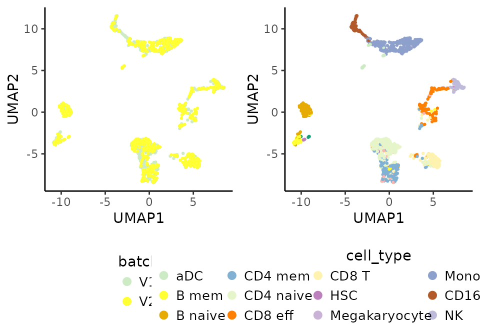
R session
# R session
sessionInfo()
## R version 4.4.2 (2024-10-31)
## Platform: x86_64-pc-linux-gnu
## Running under: Ubuntu 24.04.1 LTS
##
## Matrix products: default
## BLAS: /usr/lib/x86_64-linux-gnu/openblas-pthread/libblas.so.3
## LAPACK: /usr/lib/x86_64-linux-gnu/openblas-pthread/libopenblasp-r0.3.26.so; LAPACK version 3.12.0
##
## locale:
## [1] LC_CTYPE=C.UTF-8 LC_NUMERIC=C LC_TIME=C.UTF-8
## [4] LC_COLLATE=C.UTF-8 LC_MONETARY=C.UTF-8 LC_MESSAGES=C.UTF-8
## [7] LC_PAPER=C.UTF-8 LC_NAME=C LC_ADDRESS=C
## [10] LC_TELEPHONE=C LC_MEASUREMENT=C.UTF-8 LC_IDENTIFICATION=C
##
## time zone: UTC
## tzcode source: system (glibc)
##
## attached base packages:
## [1] stats4 stats graphics grDevices utils datasets methods
## [8] base
##
## other attached packages:
## [1] SingleCellExperiment_1.28.1 SummarizedExperiment_1.36.0
## [3] Biobase_2.66.0 GenomicRanges_1.58.0
## [5] GenomeInfoDb_1.42.3 IRanges_2.40.1
## [7] S4Vectors_0.44.0 BiocGenerics_0.52.0
## [9] MatrixGenerics_1.18.1 matrixStats_1.5.0
## [11] Coralysis_1.0.0
##
## loaded via a namespace (and not attached):
## [1] rlang_1.1.5 magrittr_2.0.3 flexclust_1.4-2
## [4] compiler_4.4.2 png_0.1-8 systemfonts_1.2.1
## [7] vctrs_0.6.5 reshape2_1.4.4 stringr_1.5.1
## [10] pkgconfig_2.0.3 crayon_1.5.3 fastmap_1.2.0
## [13] XVector_0.46.0 labeling_0.4.3 scuttle_1.16.0
## [16] rmarkdown_2.29 ggbeeswarm_0.7.2 UCSC.utils_1.2.0
## [19] ragg_1.3.3 xfun_0.50 modeltools_0.2-23
## [22] bluster_1.16.0 zlibbioc_1.52.0 cachem_1.1.0
## [25] beachmat_2.22.0 jsonlite_1.8.9 DelayedArray_0.32.0
## [28] BiocParallel_1.40.0 irlba_2.3.5.1 parallel_4.4.2
## [31] aricode_1.0.3 cluster_2.1.6 R6_2.6.0
## [34] bslib_0.9.0 stringi_1.8.4 RColorBrewer_1.1-3
## [37] reticulate_1.40.0 limma_3.62.2 jquerylib_0.1.4
## [40] Rcpp_1.0.14 iterators_1.0.14 knitr_1.49
## [43] snow_0.4-4 Matrix_1.7-1 igraph_2.1.4
## [46] tidyselect_1.2.1 abind_1.4-8 yaml_2.3.10
## [49] codetools_0.2-20 doRNG_1.8.6.1 lattice_0.22-6
## [52] tibble_3.2.1 plyr_1.8.9 withr_3.0.2
## [55] askpass_1.2.1 ggrastr_1.0.2 evaluate_1.0.3
## [58] desc_1.4.3 pillar_1.10.1 rngtools_1.5.2
## [61] foreach_1.5.2 generics_0.1.3 ggplot2_3.5.1
## [64] sparseMatrixStats_1.18.0 munsell_0.5.1 scales_1.3.0
## [67] class_7.3-22 glue_1.8.0 metapod_1.14.0
## [70] pheatmap_1.0.12 LiblineaR_2.10-24 tools_4.4.2
## [73] BiocNeighbors_2.0.1 ScaledMatrix_1.14.0 SparseM_1.84-2
## [76] RSpectra_0.16-2 locfit_1.5-9.11 RANN_2.6.2
## [79] fs_1.6.5 scran_1.34.0 Cairo_1.6-2
## [82] cowplot_1.1.3 grid_4.4.2 umap_0.2.10.0
## [85] edgeR_4.4.2 colorspace_2.1-1 GenomeInfoDbData_1.2.13
## [88] beeswarm_0.4.0 BiocSingular_1.22.0 vipor_0.4.7
## [91] cli_3.6.4 rsvd_1.0.5 textshaping_1.0.0
## [94] S4Arrays_1.6.0 dplyr_1.1.4 doSNOW_1.0.20
## [97] gtable_0.3.6 sass_0.4.9 digest_0.6.37
## [100] SparseArray_1.6.1 dqrng_0.4.1 farver_2.1.2
## [103] htmltools_0.5.8.1 pkgdown_2.1.1 lifecycle_1.0.4
## [106] httr_1.4.7 statmod_1.5.0 openssl_2.3.2References
Amezquita R, Lun A, Becht E, Carey V, Carpp L, Geistlinger L, Marini F, Rue-Albrecht K, Risso D, Soneson C, Waldron L, Pages H, Smith M, Huber W, Morgan M, Gottardo R, Hicks S (2020). “Orchestrating single-cell analysis with Bioconductor.” Nature Methods, 17, 137-145. https://www.nature.com/articles/s41592-019-0654-x.
Sousa A, Smolander J, Junttila S, Elo L (2025). “Coralysis enables sensitive identification of imbalanced cell types and states in single-cell data via multi-level integration.” bioRxiv. doi:10.1101/2025.02.07.637023