Multi-level integration — RunParallelDivisiveICP • Coralysis

Run divisive ICP clustering in parallel in order to perform multi-level integration.

Usage

RunParallelDivisiveICP.SingleCellExperiment(
  object,
  batch.label,
  k,
  d,
  L,
  r,
  C,
  reg.type,
  max.iter,
  threads,
  icp.batch.size,
  train.with.bnn,
  train.k.nn,
  train.k.nn.prop,
  build.train.set,
  build.train.params,
  scale.by,
  use.cluster.seed,
  divisive.method,
  allow.free.k,
  ari.cutoff,
  verbose
)

# S4 method for class 'SingleCellExperiment'
RunParallelDivisiveICP(
  object,
  batch.label = NULL,
  k = 16,
  d = 0.3,
  L = 50,
  r = 5,
  C = 0.3,
  reg.type = "L1",
  max.iter = 200,
  threads = 0,
  icp.batch.size = Inf,
  train.with.bnn = TRUE,
  train.k.nn = 10,
  train.k.nn.prop = 0.3,
  build.train.set = TRUE,
  build.train.params = list(),
  scale.by = NULL,
  use.cluster.seed = TRUE,
  divisive.method = "cluster.batch",
  allow.free.k = TRUE,
  ari.cutoff = 0.3,
  verbose = FALSE
)

Arguments

object: An object of SingleCellExperiment class.
batch.label: A variable name (of class character) available in the cell metadata colData(object) with the batch labels (character or factor) to use. The variable provided must not contain NAs. By default NULL, i.e., cells are sampled evenly regardless their batch.
k: A positive integer power of two, i.e., 2**n, where n>0, specifying the number of clusters in the last Iterative Clustering Projection (ICP) round. Decreasing k leads to smaller cell populations diversity and vice versa. Default is 16, i.e., the divisive clustering 2 -> 4 -> 8 -> 16 is performed.
d: A numeric greater than 0 and smaller than 1 that determines how many cells n are down- or oversampled from each cluster into the training data (n=N/k*d), where N is the total number of cells, k is the number of clusters in ICP. Increasing above 0.3 leads greadually to smaller cell populations diversity. Default is 0.3.
L: A positive integer greater than 1 denoting the number of the ICP runs to run. Default is 50. Increasing recommended with a significantly larger sample size (tens of thousands of cells). Default is 200.
r: A positive integer that denotes the number of reiterations performed until the ICP algorithm stops. Increasing recommended with a significantly larger sample size (tens of thousands of cells). Default is 5.
C: A positive real number denoting the cost of constraints violation in the L1-regularized logistic regression model from the LIBLINEAR library. Decreasing leads to more stringent feature selection, i.e. less features are selected that are used to build the projection classifier. Decreasing to a very low value (~ 0.01) can lead to failure to identify central cell populations. Default 0.3.
reg.type: "L1" or "L2". L2-regularization was not investigated in the manuscript, but it leads to a more conventional outcome (less subpopulations). Default is "L1".
max.iter: A positive integer that denotes the maximum number of iterations performed until ICP stops. This parameter is only useful in situations where ICP converges extremely slowly, preventing the algorithm to run too long. In most cases, reaching the number of reiterations (r=5) terminates the algorithm. Default is 200.
threads: A positive integer that specifies how many logical processors (threads) to use in parallel computation. Set 1 to disable parallelism altogether or 0 to use all available threas except one. Default is 0.
icp.batch.size: A positive integer that specifies how many cells to randomly select. It behaves differently depending on build.train.set. If build.train.set=FALSE, it randomly samples cells for each ICP run from the complete dataset. If build.train.set=TRUE, it randomly samples cells once, before building the training set with the sampled cells (per batch if batch.label different than NULL). Default is Inf, which means using all cells.
train.with.bnn: Train data with batch nearest neighbors. Default is TRUE. Only used if batch.label is given.
train.k.nn: Train data with batch nearest neighbors using k nearest neighbors. Default is 10. Only used if train.with.bnn is TRUE and train.k.nn.prop is NULL.
train.k.nn.prop: A numeric (higher than 0 and lower than 1) corresponding to the fraction of cells per cluster to use as train.k.nn nearest neighbors. If NULL the number of train.k.nn nearest neighbors is equal to train.k.nn. If given, train.k.nn parameter is ignored and train.k.nn is calculated based on train.k.nn.prop. By default 0.3 meaning that 30 proportions for the different divisive clustering rounds can be given, otherwise the same value is given for all.
build.train.set: Logical specifying if a training set should be built from the data or the whole data should be used for training. By default TRUE.
build.train.params: A list of parameters to be passed to the function AggregateDataByBatch(). Only provided if build.train.set is TRUE.
scale.by: A character specifying if the data should be scaled by cell or by feature before training. Default is NULL, i.e., the data is not scaled before training.
use.cluster.seed: Should the same starting clustering result be provided to ensure more reproducible results (logical). If FALSE, each ICP run starts with a total random clustering and, thus, independent clustering. By default TRUE, i.e., the same clustering result is provided based on PCA density sampling. If batch.label different than NULL, the PCA density sampling is performed in a batch wise manner.
divisive.method: Divisive method (character). One of "random" (randomly sample two clusters out of every cluster previously found), "cluster" or "cluster.batch" (sample two clusters out of every cluster previously found based on the cluster probability distribution across batches or per batch). By default "cluster.batch". If batch.label is NULL, it is automatically set to cluster. It can be set to random if explicitly provided.
allow.free.k: Allow free k (logical). Allow ICP algorithm to decrease the k given in case it does not find k target clusters. By default TRUE.
ari.cutoff: Include ICP models and probability tables with an Adjusted Rand Index higher than ari.cutoff (numeric). By default 0.3. A value that can range between 0 (include all) and lower than 1.
verbose: A logical value to print verbose during the ICP run in case of parallelization, i.e., 'threads' different than 1. Default 'FALSE'.

Value

A SingleCellExperiment object.

Examples

# Import package
suppressPackageStartupMessages(library("SingleCellExperiment"))

# Create toy SCE data
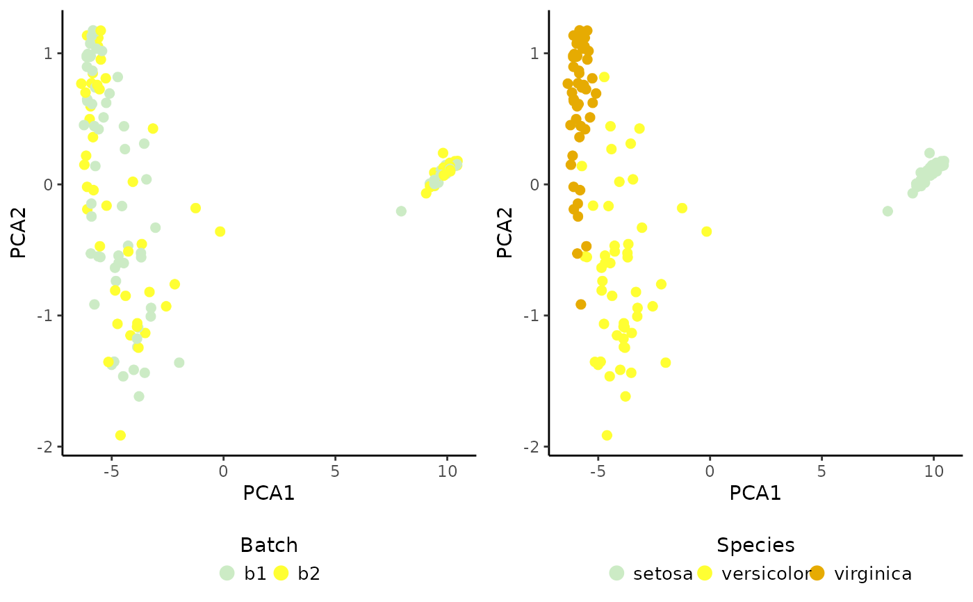
batches <- c("b1", "b2")
set.seed(239)
batch <- sample(x = batches, size = nrow(iris), replace = TRUE)
sce <- SingleCellExperiment(assays = list(logcounts = t(iris[,1:4])),  
                            colData = DataFrame("Species" = iris$Species, 
                                               "Batch" = batch))
colnames(sce) <- paste0("samp", 1:ncol(sce))

# Prepare SCE object for analysis
sce <- PrepareData(sce)
#> Converting object of `matrix` class into `dgCMatrix`. Please note that Coralysis has been designed to work with sparse data, i.e. data with a high proportion of zero values! Dense data will likely increase run time and memory usage drastically!
#> 4/4 features remain after filtering features with only zero values.

# Multi-level integration (just for highlighting purposes; use default parameters)
set.seed(123)
sce <- RunParallelDivisiveICP(object = sce, batch.label = "Batch", 
                              k = 2, L = 25, C = 1, train.k.nn = 10, 
                              train.k.nn.prop = NULL, use.cluster.seed = FALSE,
                              build.train.set = FALSE, ari.cutoff = 0.1, 
                              threads = 2)
#> 
#> Initializing divisive ICP clustering...
#> 
  |                                                                            
  |                                                                      |   0%
  |                                                                            
  |===                                                                   |   4%
  |                                                                            
  |======                                                                |   8%
  |                                                                            
  |=========                                                             |  12%
  |                                                                            
  |============                                                          |  17%
  |                                                                            
  |===============                                                       |  21%
  |                                                                            
  |==================                                                    |  25%
  |                                                                            
  |====================                                                  |  29%
  |                                                                            
  |=======================                                               |  33%
  |                                                                            
  |==========================                                            |  38%
  |                                                                            
  |=============================                                         |  42%
  |                                                                            
  |================================                                      |  46%
  |                                                                            
  |===================================                                   |  50%
  |                                                                            
  |======================================                                |  54%
  |                                                                            
  |=========================================                             |  58%
  |                                                                            
  |============================================                          |  62%
  |                                                                            
  |===============================================                       |  67%
  |                                                                            
  |==================================================                    |  71%
  |                                                                            
  |====================================================                  |  75%
  |                                                                            
  |=======================================================               |  79%
  |                                                                            
  |==========================================================            |  83%
  |                                                                            
  |=============================================================         |  88%
  |                                                                            
  |================================================================      |  92%
  |                                                                            
  |===================================================================   |  96%
  |                                                                            
  |======================================================================| 100%
#> 
#> Divisive ICP clustering completed successfully.
#> 
#> Predicting cell cluster probabilities using ICP models...
#> Prediction of cell cluster probabilities completed successfully.
#> 
#> Multi-level integration completed successfully.

# Integrated PCA
set.seed(125) # to ensure reproducibility for the default 'irlba' method
sce <- RunPCA(object = sce, assay.name = "joint.probability", p = 10)
#> Divisive ICP: selecting ICP tables multiple of 1

# Plot result 
cowplot::plot_grid(PlotDimRed(object = sce, color.by = "Batch", 
                              legend.nrow = 1),
                   PlotDimRed(object = sce, color.by = "Species", 
                              legend.nrow = 1), ncol = 2)