Run nonlinear dimensionality reduction using UMAP with a dimensional reduction as input.
Usage
RunUMAP.SingleCellExperiment(
  object,
  dims,
  dimred.type,
  return.model,
  umap.method,
  dimred.name,
  ...
)

# S4 method for class 'SingleCellExperiment'
RunUMAP(
  object,
  dims = NULL,
  dimred.type = "PCA",
  return.model = FALSE,
  umap.method = "umap",
  dimred.name = "UMAP",
  ...
)
Arguments
- object
An object of
SingleCellExperimentclass.- dims
Dimensions to select from
dimred.type. By defaultNULL, i.e., all the dimensions are selected. Provide a numeric vector to select a specific range, e.g.,dims = 1:10to select the first 10 dimensions.- dimred.type
Dimensional reduction type to use. By default
"PCA".- return.model
Return UMAP model. By default
FALSE.- umap.method
UMAP method to use:
"umap"or"uwot". By default"umap".- dimred.name
Dimensional reduction name given to the returned UMAP. By default
"UMAP".- ...
Parameters to be passed to the
umapfunction. The parameters given should match the parameters accepted by theumapfunction depending on theumap.methodgiven. Check possible parameters with?umap::umapor?uwot::umapdepending ifumap.methodis"umap"or"uwot".
Examples
# Import package
suppressPackageStartupMessages(library("SingleCellExperiment"))
# Create toy SCE data
batches <- c("b1", "b2")
set.seed(239)
batch <- sample(x = batches, size = nrow(iris), replace = TRUE)
sce <- SingleCellExperiment(assays = list(logcounts = t(iris[,1:4])),
colData = DataFrame("Species" = iris$Species,
"Batch" = batch))
colnames(sce) <- paste0("samp", 1:ncol(sce))
# Prepare SCE object for analysis
sce <- PrepareData(sce)
#> Converting object of `matrix` class into `dgCMatrix`. Please note that Coralysis has been designed to work with sparse data, i.e. data with a high proportion of zero values! Dense data will likely increase run time and memory usage drastically!
#> 4/4 features remain after filtering features with only zero values.
# Multi-level integration (just for highlighting purposes; use default parameters)
set.seed(123)
sce <- RunParallelDivisiveICP(object = sce, batch.label = "Batch",
k = 2, L = 25, C = 1, train.k.nn = 10,
train.k.nn.prop = NULL, use.cluster.seed = FALSE,
build.train.set = FALSE, ari.cutoff = 0.1,
threads = 2)
#>
#> Initializing divisive ICP clustering...
#>
|
| | 0%
|
|=== | 4%
|
|====== | 8%
|
|========= | 12%
|
|============ | 17%
|
|=============== | 21%
|
|================== | 25%
|
|==================== | 29%
|
|======================= | 33%
|
|========================== | 38%
|
|============================= | 42%
|
|================================ | 46%
|
|=================================== | 50%
|
|====================================== | 54%
|
|========================================= | 58%
|
|============================================ | 62%
|
|=============================================== | 67%
|
|================================================== | 71%
|
|==================================================== | 75%
|
|======================================================= | 79%
|
|========================================================== | 83%
|
|============================================================= | 88%
|
|================================================================ | 92%
|
|=================================================================== | 96%
|
|======================================================================| 100%
#>
#> Divisive ICP clustering completed successfully.
#>
#> Predicting cell cluster probabilities using ICP models...
#> Prediction of cell cluster probabilities completed successfully.
#>
#> Multi-level integration completed successfully.
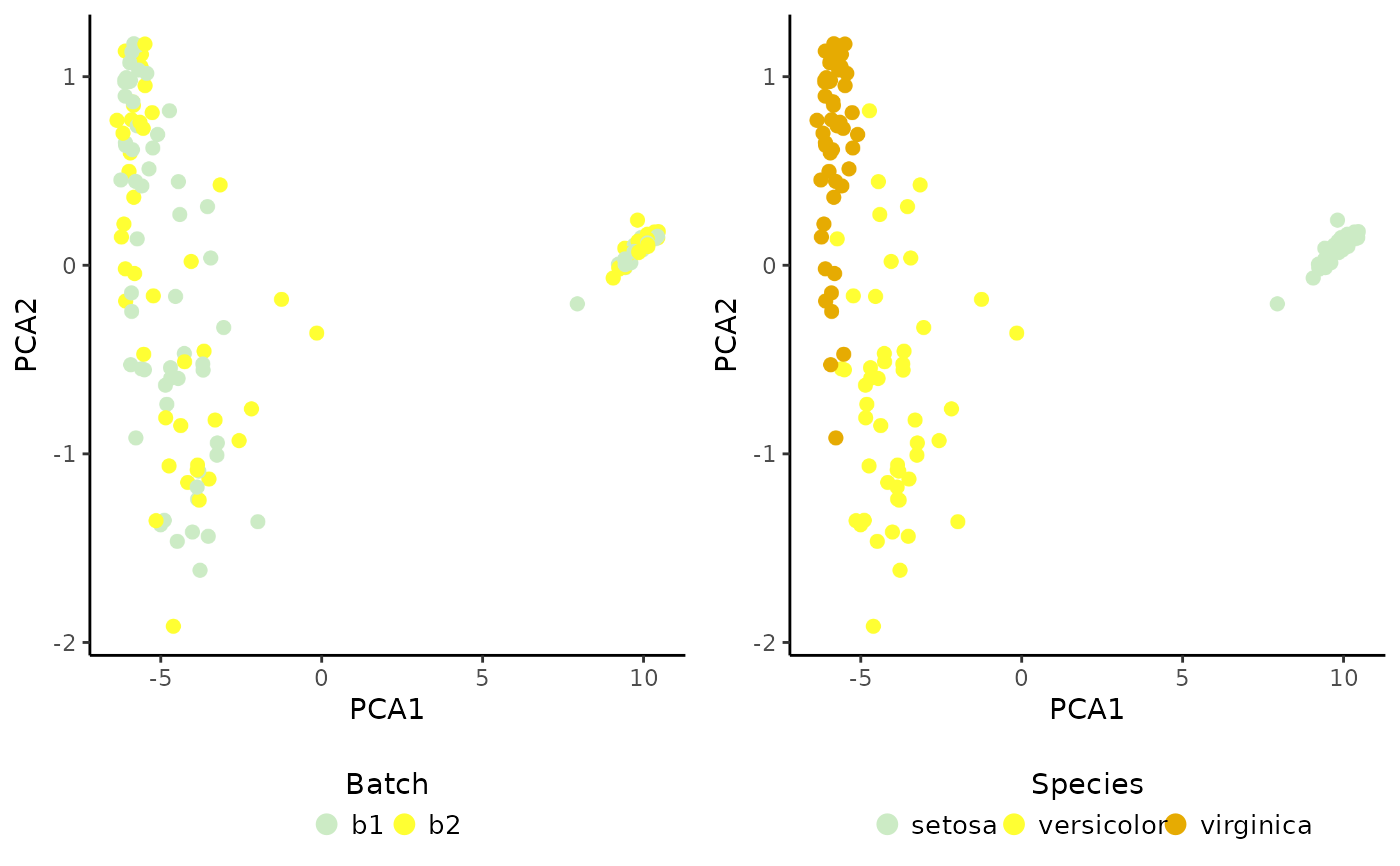
# Integrated PCA
set.seed(125) # to ensure reproducibility for the default 'irlba' method
sce <- RunPCA(object = sce, assay.name = "joint.probability", p = 10)
#> Divisive ICP: selecting ICP tables multiple of 1
# Plot result
cowplot::plot_grid(PlotDimRed(object = sce, color.by = "Batch",
legend.nrow = 1),
PlotDimRed(object = sce, color.by = "Species",
legend.nrow = 1), ncol = 2)
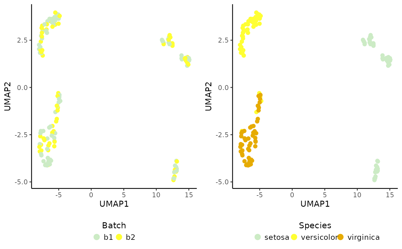
 # Run UMAP
set.seed(123)
sce <- RunUMAP(sce, dimred.type = "PCA")
# Plot results
# Plot result
cowplot::plot_grid(PlotDimRed(object = sce, color.by = "Batch",
legend.nrow = 1),
PlotDimRed(object = sce, color.by = "Species",
legend.nrow = 1), ncol = 2)
# Run UMAP
set.seed(123)
sce <- RunUMAP(sce, dimred.type = "PCA")
# Plot results
# Plot result
cowplot::plot_grid(PlotDimRed(object = sce, color.by = "Batch",
legend.nrow = 1),
PlotDimRed(object = sce, color.by = "Species",
legend.nrow = 1), ncol = 2)