Summarise ICP cell cluster probability — SummariseCellClusterProbability • Coralysis

Summarise ICP cell cluster probability table(s)

Usage

SummariseCellClusterProbability.SingleCellExperiment(
  object,
  icp.run,
  icp.round,
  funs,
  scale.funs,
  save.in.sce
)

# S4 method for class 'SingleCellExperiment'
SummariseCellClusterProbability(
  object,
  icp.run = NULL,
  icp.round = NULL,
  funs = c("mean", "median"),
  scale.funs = TRUE,
  save.in.sce = TRUE
)

Arguments

object: An object of SingleCellExperiment class with ICP cell cluster probability tables saved in metadata(object)$coralysis$joint.probability. After running RunParallelDivisiveICP.
icp.run: ICP run(s) to retrieve from metadata(object)$coralysis$joint.probability. By default NULL, i.e., all are retrieved. Specify a numeric vector to retrieve a specific set of tables.
icp.round: ICP round(s) to retrieve from metadata(object)$coralysis$joint.probability. By default NULL, i.e., all are retrieved.
funs: Functions to summarise ICP cell cluster probability: "mean" and/or "median". By default c("mean", "median"), i.e, both mean and median are calculated. Set to NULL to not estimate any.
scale.funs: Scale in the range 0-1 the summarised probability obtained with funs. By default TRUE, i.e., summarised probability will be scaled in the 0-1 range.
save.in.sce: Save the data frame into the cell metadata from the SingleCellExperiment object or return the data frame. By default TRUE, i.e., the summary of probabilities retrieved is save in the SCE object in colData(object).

Value

A data frame or a SingleCellExperiment object with ICP cell cluster probability summarised.

Examples

# Import package
suppressPackageStartupMessages(library("SingleCellExperiment"))

# Create toy SCE data
batches <- c("b1", "b2")
set.seed(239)
batch <- sample(x = batches, size = nrow(iris), replace = TRUE)
sce <- SingleCellExperiment(assays = list(logcounts = t(iris[,1:4])),  
                            colData = DataFrame("Species" = iris$Species, 
                                               "Batch" = batch))
colnames(sce) <- paste0("samp", 1:ncol(sce))

# Prepare SCE object for analysis
sce <- PrepareData(sce)
#> Converting object of `matrix` class into `dgCMatrix`. Please note that Coralysis has been designed to work with sparse data, i.e. data with a high proportion of zero values! Dense data will likely increase run time and memory usage drastically!
#> 4/4 features remain after filtering features with only zero values.

# Multi-level integration (just for highlighting purposes; use default parameters)
set.seed(123)
sce <- RunParallelDivisiveICP(object = sce, batch.label = "Batch", 
                              k = 2, L = 25, C = 1, train.k.nn = 10, 
                              train.k.nn.prop = NULL, use.cluster.seed = FALSE,
                              build.train.set = FALSE, ari.cutoff = 0.1, 
                             threads = 2)
#> 
#> Initializing divisive ICP clustering...
#> 
  |                                                                            
  |                                                                      |   0%
  |                                                                            
  |===                                                                   |   4%
  |                                                                            
  |======                                                                |   8%
  |                                                                            
  |=========                                                             |  12%
  |                                                                            
  |============                                                          |  17%
  |                                                                            
  |===============                                                       |  21%
  |                                                                            
  |==================                                                    |  25%
  |                                                                            
  |====================                                                  |  29%
  |                                                                            
  |=======================                                               |  33%
  |                                                                            
  |==========================                                            |  38%
  |                                                                            
  |=============================                                         |  42%
  |                                                                            
  |================================                                      |  46%
  |                                                                            
  |===================================                                   |  50%
  |                                                                            
  |======================================                                |  54%
  |                                                                            
  |=========================================                             |  58%
  |                                                                            
  |============================================                          |  62%
  |                                                                            
  |===============================================                       |  67%
  |                                                                            
  |==================================================                    |  71%
  |                                                                            
  |====================================================                  |  75%
  |                                                                            
  |=======================================================               |  79%
  |                                                                            
  |==========================================================            |  83%
  |                                                                            
  |=============================================================         |  88%
  |                                                                            
  |================================================================      |  92%
  |                                                                            
  |===================================================================   |  96%
  |                                                                            
  |======================================================================| 100%
#> 
#> Divisive ICP clustering completed successfully.
#> 
#> Predicting cell cluster probabilities using ICP models...
#> Prediction of cell cluster probabilities completed successfully.
#> 
#> Multi-level integration completed successfully.
                             
# Integrated PCA
set.seed(125) # to ensure reproducibility for the default 'irlba' method
sce <- RunPCA(object = sce, assay.name = "joint.probability", p = 10)
#> Divisive ICP: selecting ICP tables multiple of 1

# Summarise cluster probability
sce <- SummariseCellClusterProbability(object = sce, icp.round = 1, 
                                       save.in.sce = TRUE) # saved in 'colData'

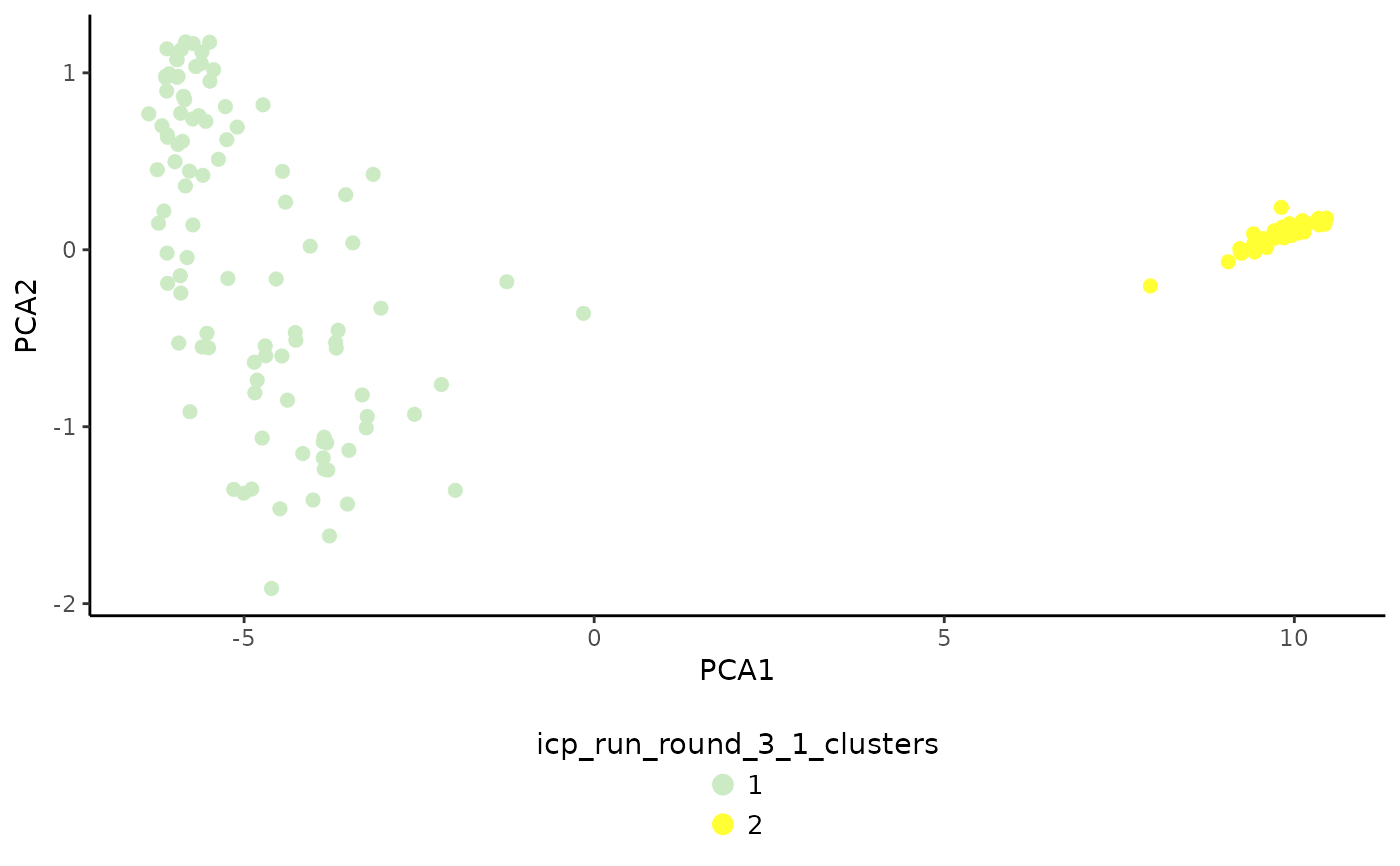
# Plot the clustering result for ICP run no. 3 
PlotDimRed(object = sce, color.by = "icp_run_round_3_1_clusters")


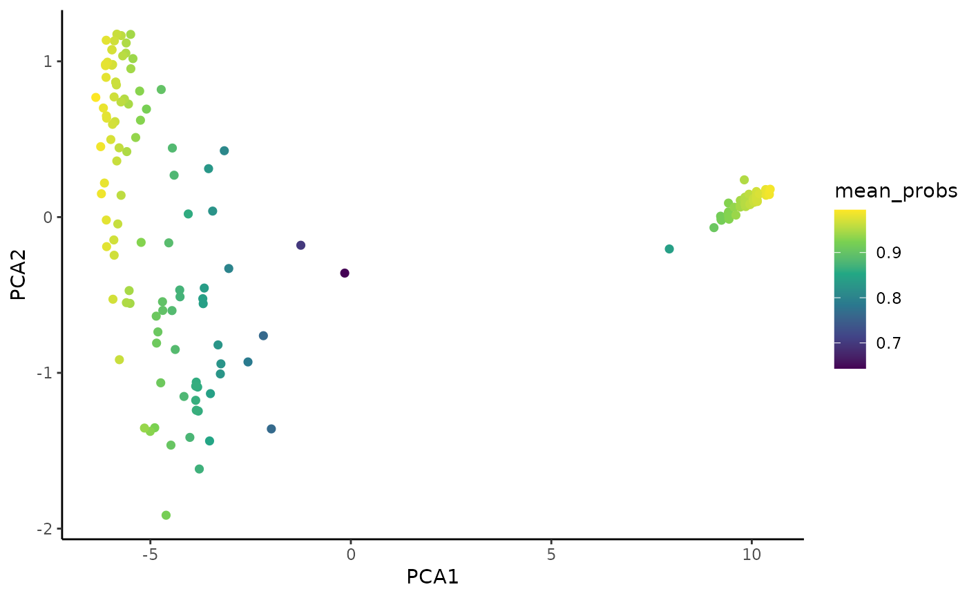
# Plot Coralysis mean cell cluster probabilities 
PlotExpression(object = sce, color.by = "mean_probs", 
               color.scale = "viridis")