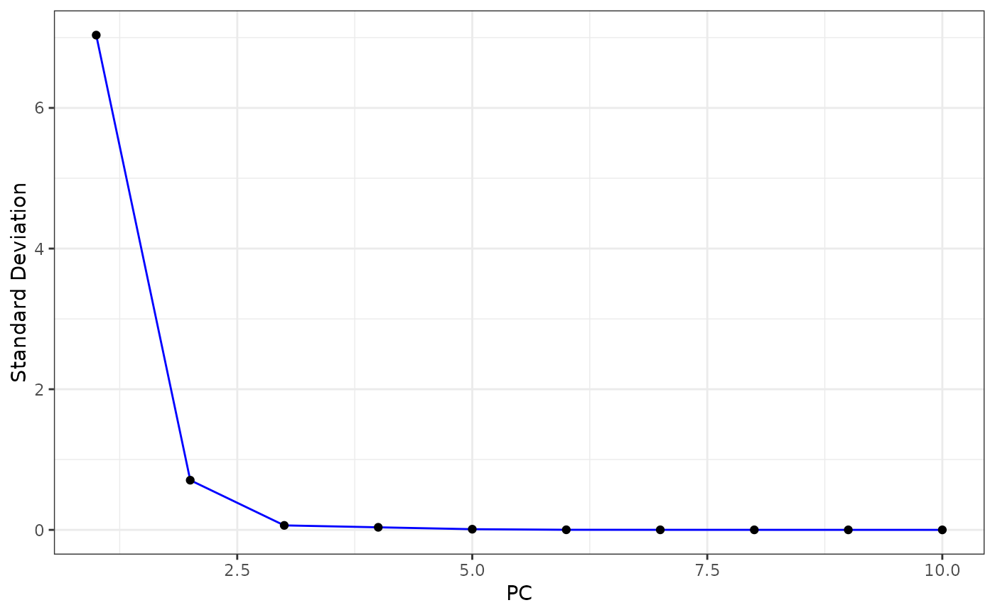
Elbow plot of the standard deviations of the principal components

Draw an elbow plot of the standard deviations of the principal components to deduce an appropriate value for p.

Usage

PCAElbowPlot.SingleCellExperiment(object, dimred.name, return.plot)

# S4 method for class 'SingleCellExperiment'
PCAElbowPlot(object, dimred.name = "PCA", return.plot = FALSE)

Arguments

object

A SingleCellExperiment object obtained after running RunParallelDivisiveICP.

dimred.name

Dimensional reduction name of the PCA to select from reducedDimNames(object). By default "PCA".

return.plot

logical indicating if the ggplot2 object should be returned. By default FALSE.

Value

A ggplot2 object, if return.plot=TRUE.

Examples

# Import package
suppressPackageStartupMessages(library("SingleCellExperiment"))

# Create toy SCE data
batches <- c("b1", "b2")
set.seed(239)
batch <- sample(x = batches, size = nrow(iris), replace = TRUE)
sce <- SingleCellExperiment(assays = list(logcounts = t(iris[,1:4])),  
                            colData = DataFrame("Species" = iris$Species, 
                                               "Batch" = batch))
colnames(sce) <- paste0("samp", 1:ncol(sce))

# Prepare SCE object for analysis
sce <- PrepareData(sce)
#> Converting object of `matrix` class into `dgCMatrix`. Please note that Coralysis has been designed to work with sparse data, i.e. data with a high proportion of zero values! Dense data will likely increase run time and memory usage drastically!
#> 4/4 features remain after filtering features with only zero values.

# Multi-level integration (just for highlighting purposes; use default parameters)
set.seed(123)
sce <- RunParallelDivisiveICP(object = sce, batch.label = "Batch", 
                              k = 2, L = 25, C = 1, train.k.nn = 10, 
                              train.k.nn.prop = NULL, use.cluster.seed = FALSE,
                              build.train.set = FALSE, ari.cutoff = 0.1, 
                             threads = 2)
#> 
#> Initializing divisive ICP clustering...
#> 
  |                                                                            
  |                                                                      |   0%
  |                                                                            
  |===                                                                   |   4%
  |                                                                            
  |======                                                                |   8%
  |                                                                            
  |=========                                                             |  12%
  |                                                                            
  |============                                                          |  17%
  |                                                                            
  |===============                                                       |  21%
  |                                                                            
  |==================                                                    |  25%
  |                                                                            
  |====================                                                  |  29%
  |                                                                            
  |=======================                                               |  33%
  |                                                                            
  |==========================                                            |  38%
  |                                                                            
  |=============================                                         |  42%
  |                                                                            
  |================================                                      |  46%
  |                                                                            
  |===================================                                   |  50%
  |                                                                            
  |======================================                                |  54%
  |                                                                            
  |=========================================                             |  58%
  |                                                                            
  |============================================                          |  62%
  |                                                                            
  |===============================================                       |  67%
  |                                                                            
  |==================================================                    |  71%
  |                                                                            
  |====================================================                  |  75%
  |                                                                            
  |=======================================================               |  79%
  |                                                                            
  |==========================================================            |  83%
  |                                                                            
  |=============================================================         |  88%
  |                                                                            
  |================================================================      |  92%
  |                                                                            
  |===================================================================   |  96%
  |                                                                            
  |======================================================================| 100%
#> 
#> Divisive ICP clustering completed successfully.
#> 
#> Predicting cell cluster probabilities using ICP models...
#> Prediction of cell cluster probabilities completed successfully.
#> 
#> Multi-level integration completed successfully.

# Integrated PCA
set.seed(125) # to ensure reproducibility for the default 'irlba' method
sce <- RunPCA(object = sce, assay.name = "joint.probability", p = 10)
#> Divisive ICP: selecting ICP tables multiple of 1

# Plot result 
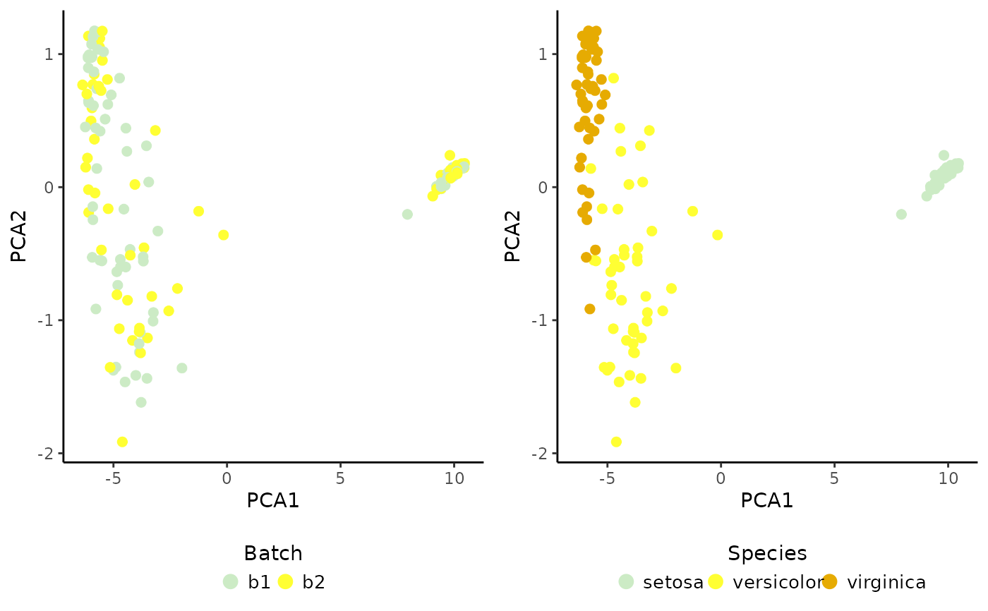
cowplot::plot_grid(PlotDimRed(object = sce, color.by = "Batch", 
                              legend.nrow = 1),
                   PlotDimRed(object = sce, color.by = "Species", 
                             legend.nrow = 1), ncol = 2)


# Plot Elbow
PCAElbowPlot(sce)