Plot cluster tree by or cluster probability or categorical variable.
Usage
PlotClusterTree.SingleCellExperiment(
  object,
  icp.run,
  color.by,
  use.color,
  seed.color,
  legend.title,
  return.data
)

# S4 method for class 'SingleCellExperiment'
PlotClusterTree(
  object,
  icp.run,
  color.by = NULL,
  use.color = NULL,
  seed.color = 123,
  legend.title = color.by,
  return.data = FALSE
)
Arguments
- object
An object of
SingleCellExperimentclass.- icp.run
ICP run(s) to retrieve from
metadata(object)$coralysis$joint.probability. By defaultNULL, i.e., all are retrieved. Specify a numeric vector to retrieve a specific set of tables.- color.by
Categorical variable available in
colData(object)to plot. IfNULLthe cluster probability is represented instead. By defaultNULL.- use.color
Character specifying the colors. By default
NULL, i.e., colors are randomly chosen based on the seed given atseed.color.- seed.color
Seed to randomly select colors. By default
123.- legend.title
Legend title. By default the same as given at
color.by. Ignored ifcolor.byisNULL.- return.data
Return data frame used to plot. Logical. By default
FALSE, i.e., only the plot is returned.
Examples
# Import package
suppressPackageStartupMessages(library("SingleCellExperiment"))
# Create toy SCE data
batches <- c("b1", "b2")
set.seed(239)
batch <- sample(x = batches, size = nrow(iris), replace = TRUE)
sce <- SingleCellExperiment(assays = list(logcounts = t(iris[,1:4])),
colData = DataFrame("Species" = iris$Species,
"Batch" = batch))
colnames(sce) <- paste0("samp", 1:ncol(sce))
# Prepare SCE object for analysis
sce <- PrepareData(sce)
#> Converting object of `matrix` class into `dgCMatrix`. Please note that Coralysis has been designed to work with sparse data, i.e. data with a high proportion of zero values! Dense data will likely increase run time and memory usage drastically!
#> 4/4 features remain after filtering features with only zero values.
# Multi-level integration (just for highlighting purposes; use default parameters)
set.seed(123)
sce <- RunParallelDivisiveICP(object = sce, batch.label = "Batch", k = 4,
L = 25, C = 1, d = 0.5, train.with.bnn = FALSE,
use.cluster.seed = FALSE, build.train.set = FALSE,
ari.cutoff = 0.1, threads = 2)
#>
#> Initializing divisive ICP clustering...
#>
|
| | 0%
|
|=== | 4%
|
|====== | 8%
|
|========= | 12%
|
|============ | 17%
|
|=============== | 21%
|
|================== | 25%
|
|==================== | 29%
|
|======================= | 33%
|
|========================== | 38%
|
|============================= | 42%
|
|================================ | 46%
|
|=================================== | 50%
|
|====================================== | 54%
|
|========================================= | 58%
|
|============================================ | 62%
|
|=============================================== | 67%
|
|================================================== | 71%
|
|==================================================== | 75%
|
|======================================================= | 79%
|
|========================================================== | 83%
|
|============================================================= | 88%
|
|================================================================ | 92%
|
|=================================================================== | 96%
|
|======================================================================| 100%
#>
#> Divisive ICP clustering completed successfully.
#>
#> Predicting cell cluster probabilities using ICP models...
#> Prediction of cell cluster probabilities completed successfully.
#>
#> Multi-level integration completed successfully.
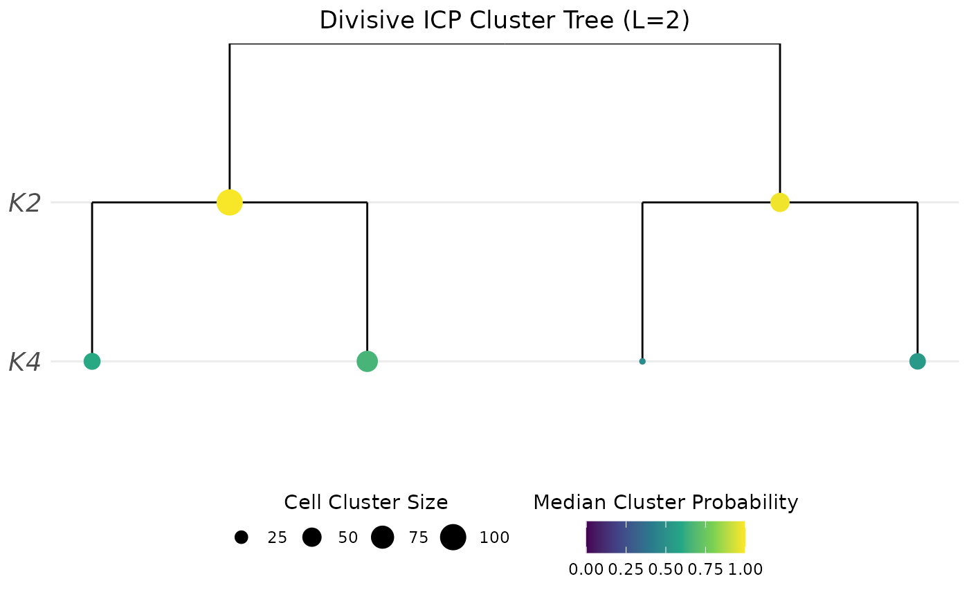
# Plot probability
PlotClusterTree(object = sce, icp.run = 2)
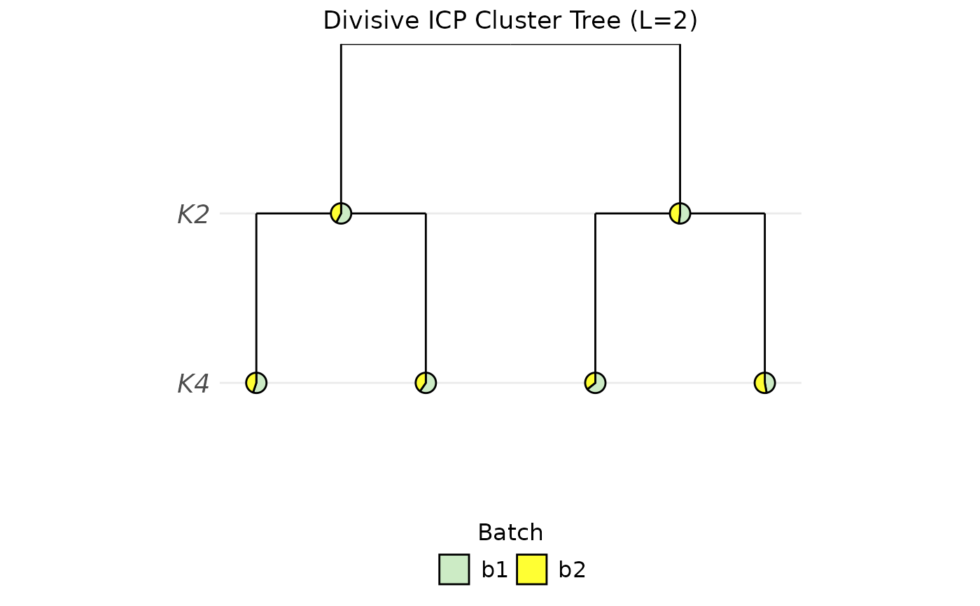
 # Plot batch label distribution
PlotClusterTree(object = sce, icp.run = 2, color.by = "Batch")
# Plot batch label distribution
PlotClusterTree(object = sce, icp.run = 2, color.by = "Batch")
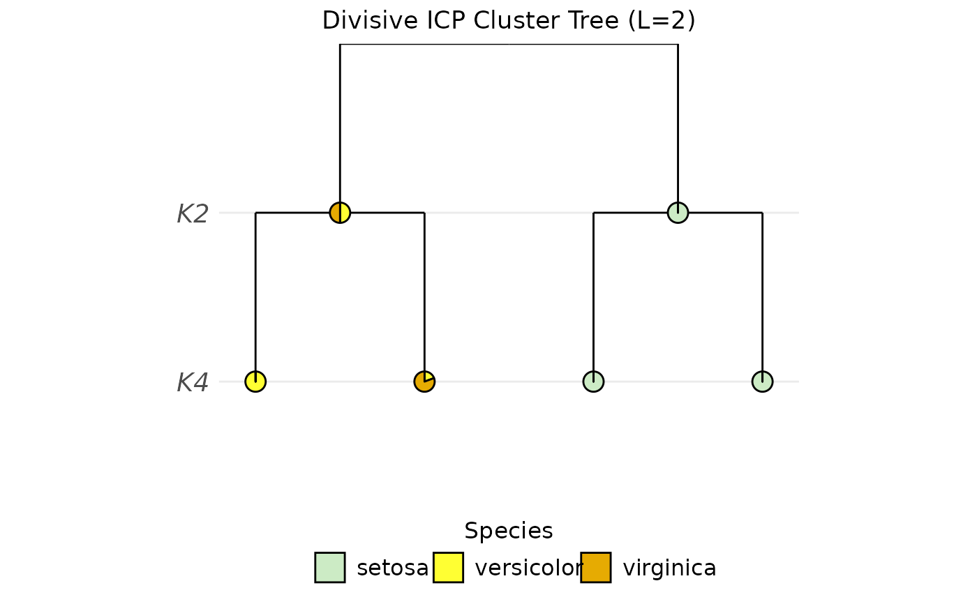
 # Plot species label distribution
PlotClusterTree(object = sce, icp.run = 2, color.by = "Species")
# Plot species label distribution
PlotClusterTree(object = sce, icp.run = 2, color.by = "Species")